Quandle $2$-Cocycle Invariants of Classical Knots

The cocycle invariant for classical knots [CJKLS03] using quandle $2$-cocycles was defined as follows. Let $X$ be a finite quandle and $A$ an abelian group.

A function $\phi : X \times X \rightarrow A$ is called a quandle $2$-cocycle if it satisfies the $2$-cocycle condition

$$\phi(x,y) - \phi(x,z) + \phi(x*y, z) - \phi(x*z, y*z)=0,$$

for all $x,y,z \in X$ and $\phi(x,x)=0$ for all $x \in X$. Let ${\mathcal C}$ be a coloring of a given diagram $D$ of a knot $K$ by $X$. The $($Boltzmann$)$ weight $B( {\mathcal C}, \tau)$ at a crossing $\tau$ of $K$ is then defined by $B( {\mathcal C}, \tau)=\phi(x_{\tau}, y_{\tau})^{\epsilon(\tau)}$, where $(x_{\tau}$, $y_{\tau})$ is the ordered pair of colors (source colors) at $\tau$ and $\epsilon(\tau)$ is the sign ($\pm 1$ for positive and negative crossings, respectively) of $\tau$. Here $B( {\mathcal C}, \tau)$ is an element of $A$ written multiplicatively. In Fig.  of Chapter $2$, if the under-arc of the crossing $\tau$ depicted is oriented downwards from $\alpha$ to $\gamma$, then $\epsilon(\tau)=1$, and $B( {\mathcal C}, \tau)=\phi(a,b)$ with the indicated coloring. If the orientation of the under-arc is opposite, then $B( {\mathcal C}, \tau)=\phi(a,b)^{-1}$.

Definition 4.1 ([CJKLS03])   The formal sum (called a state-sum) in the group ring $\mathbb{Z}[A]$

$$\Phi_{\phi} (K) = \sum_{{\mathcal C}\in {\rm Col_X(D)}} \prod_{\tau} B( {\mathcal C}, \tau )$$

is called the quandle $2$-cocycle invariant.

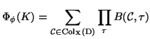
The value (an element of $\mathbb{Z}[A]$) of the invariant is written as $\sum_{g \in G} a_g g$, so that if $A=\mathbb{Z}_n=\{ u^k \vert 0 \leq k < n \}$, the value is written as a polynomial $\sum_{k=0}^{n-1} a_k u^k$. The fact that $\Phi_{\phi} (K)$ is a knot invariant is proved easily by checking Reidemeister moves [CJKLS03]. For example, in Fig.  of Chapter $2$, the product of weights that appear in the LHS is $\phi(x,y) \phi(x*y, z) \phi(y,z)$ from the top to bottom crossings, and for the RHS it is $\phi(y,z)\phi(x,z) \phi(x*z, y*z)$, and the equality obtained is exactly the $2$-cocycle condition in multiplicative notation, after canceling $\phi(y,z)$.

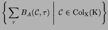
The cocycle invariant can be also written as a family (multi-set, a set with repetition allowed) of weight sums [Lop03]

$$\left\{ \left. \sum_{\tau} B_A( {\mathcal C}, \tau ) \right\vert {\mathcal C}\in {\rm Col_X(K)} \right\}$$

where now the values of $B$ in $A$ are denoted by additive notation, $B_A( {\mathcal C}, \tau ) = {\epsilon(\tau) } \phi(x_{\tau}, y_{\tau})$. Then this is well-defined for any quandle of any cardinality. The sum of the value of the weight for a specific coloring is also called the contribution of the coloring to the invariant.

The $2$-cocycle invariant is well-defined for virtual knots, as checked in a similar manner.

Example 4.2   Consider a trefoil $K$ represented by the closure of the braid $(\sigma_1)^3$, where we denote the standard braid generator by $\sigma_i$, which is represented by a positive crossing placed between $i\/$th and $(i+1)\/$st strings.

Let $X=A=\mathbb{Z}_2[t]/(t^2+t+1)$, an Alexander quandle as $X$ and an abelian group as $A$, and put the source colors $(1,0)$, for example, at the top crossing. This color vector goes down to the next crossing, giving $(0, t)$, $(t, t(1+t))$=$(t, 1)$, and comes back to $(1, t^2 + t+1)=(1,0)$, by the coloring rule, and defines a non-trivial coloring ${\mathcal C}$. In fact any pair extends to a coloring, and $\vert{\rm Col}_X(K)\vert=4^2$.

Consider the function $\phi : X \times X \rightarrow A$ defined by $\phi(x,y)=(x-y)^2 y$. Then this satisfies the $2$-cocycle condition by calculation (we will further discuss this method of construction of $2$-cocycles later).

The contribution is computed by

$$\sum_{\tau} B_A( {\mathcal C}, \tau )= 0 + (-t)^2 t + (t-1)^2 = t+1 \in A,$$

and after we compute it for all colorings, we obtain, as a multiset,

$$\Phi_\phi(K)=\{ \sqcup_4 (0) , \sqcup_{12} (t+1) \} ,$$

where $\sqcup_n x$ denotes $n$ copies of $x$ for a positive integer $n$.

We make the following notational convention. In the above example, if we denote additive generators $1$ and $t$ multiplicatively by $h$ and $k$, then the elements of $X$ in multiplicative notation are written as $\{ 1, h, k, hk \}$. Hence the invariant in the state-sum form is written as $\Phi_\phi (K)=4 + 12 hk$. In Maple calculations, it is convenient and easier to see outputs if we use the symbols $u(=u^1)$ and $u^t$ for $h$ and $k$. Then the additive notations remain on superscripts and the addition is also retained in exponents ( $hk=u \cdot u^t=u^{(t+1)}$). With this convention the invariant value is written as $4+12 u^{(t+1)}$. We use this notation if there is no confusion.